Std New Table: Difference between revisions
(Created page with "{{Docnav |Std New |Std New Matrix |Std File Menu |IconL=Std_New.svg |IconR=Std_New_Matrix.svg |IconC=Labrps.svg }} {{GuiCommand |Name=Std File New table |MenuLocation=File → New Table |Phenomena=All |Shortcut={{KEY|Ctrl}}+{{KEY|T}} |Version=0.1 |SeeAlso=Std New, Std New Matrix }} ==Description== The '''Std File New Table''' command creates new table. ==Usage== #There are several ways t...") |
No edit summary |
||
| (One intermediate revision by the same user not shown) | |||
| Line 9: | Line 9: | ||
{{GuiCommand | {{GuiCommand | ||
|Name=Std | |Name=Std New Table | ||
|MenuLocation=File → New Table | |MenuLocation=File → New Table | ||
|Phenomena=All | |Phenomena=All | ||
| Line 19: | Line 19: | ||
==Description== | ==Description== | ||
The '''Std | The '''Std New Table''' command creates new table. | ||
==Usage== | ==Usage== | ||
| Line 28: | Line 28: | ||
==Note== | ==Note== | ||
It creates a new (empty) table and adds it to the project. The empty table will have 30 rows and 2 columns. | It creates a new (empty) table and adds it to the project. The empty table will have 30 rows and 2 columns. A LabRPS Table is similar in appearance to a spreadsheet, but it differs in some important ways. In a spreadsheet, operations are performed on cells or on a range of cells. The cell is the basic unit being operated on. Row and column groupings have no inherent significance. Any relationship between observations in a spreadsheet row or column is created by the user. | ||
In contrast, Tables in LabRPS more closely mimic a flat-file database, in that each row is essentially a record with each cell in that row sharing a common row index number that groups those cells together. So, for instance, the row index number might identify an individual, and each cell in that row might contain a measurement on a different variable associated with that individual. Thus, there exists an underlying association among cells within a row, independent of any explicit association that might be conceived of by the user. | |||
Likewise -- extending the database metaphor -- each cell in the table column contains a measurement on a single variable, creating an inherent relationship among cells within a column. This column of measurements on a single variable serves to define the LabRPS Table dataset. | |||
[[File:Table.png|center]] | |||
=Columns= | |||
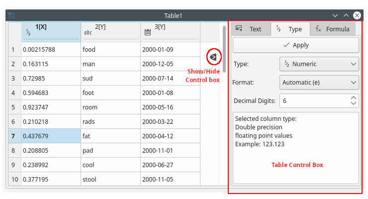
A table column can be considered as an equivalent of one-dimensional data array. Every column of the table has a set of editable predefined properties: name label, data type, data format, and a column flag. Each column properties can be changed by selecting the column and editing the property via the table control box (Table -> Show/Hide Controls). | |||
==Name== | |||
You can edit the displayed column name by clicking Text on the control box tab and entering a new name. A detailed comment on the column can also be entered if needed or leave it blank. Columns are named as numbers by default in order of their creation. Each column should have a unique name different from the name of any other columns. | |||
==Type== | |||
Each Column has a type associated with it namely: Number, Text, or Datetime. This can be changed by selecting the desired column and changing the type combo box from the control box type tab. | |||
[[File:Table_type.png|center]] | |||
==Format== | |||
Once the type is selected formatting of the type can be achieved using format option from the control box type tab. For eg number type can have a decimal, scientific(e), or auto-formatting. Datetime type can have predefined or custom formatting based on [https://doc.qt.io/archives/qt-5.11/qdatetime.html QDateTime Class] format options. | |||
==Flag== | |||
Columns can be assigned the following flags: X, Y, Z, X-error, Y-error or can be simple columns without any special flag(None). The X columns are abscissae columns while the Y columns are ordinate columns used when creating a 2D plot from data. The Z columns are used for 3D plots. The X-error and Y-error columns can be used in order to add error bars to 2D plots. | |||
[[File:Table_flag.png|center]] | |||
The line color in the column header also represents the flag X(green), Y(brown), Z(violet), X-error/y-error(red), none(grey). | |||
==Type/Format Lock== | |||
The assigned flag or type will be locked(depicted by the lock symbol along with the type icon) once you use the column for 2D or 3D plots. After locking, the user will not be allowed to change the type/format unless the plot associated with the column doesn't exist anymore. | |||
[[File:Table_type_lock.png|center]] | |||
=Operations= | |||
You can select all the columns of the spreadsheet (Ctrl+A) or only some of them by clicking on the column label while keeping the Ctrl key pressed, or by moving the mouse over the column label. This also allows you to deselect columns. | |||
On the selected columns you can perform various operations: | |||
* Fill with data. You can insert the row numbers (Fill Selection With→Row Numbers command), random numbers (Fill Selection With→Random Values command), custom random numbers(Fill Selection With→Custom Random Values command and select Gaussian, Laplace, Exponential distributions etc), or the result of a function (Assign Formula command); | |||
* normalize columns with the Normalize Columns command of the context menu; | |||
* sort columns with the Sort Table command of the Table menu or with the sort column command of the context menu; | |||
* compute statistical data on columns and rows with the Statistics on Columns command and Statistics on Rows command of the Analysis-tables menu; | |||
* build a plot from selected columns with the plot command of the context menu or with the commands of the Plot menu | |||
All these functions can be reached by right-clicking when a column is selected. Most of them can also be reached by using the Table menu. | |||
You can cut, copy and paste data between spreadsheets or between a spreadsheet and another application (Excel, Gnumeric, OpenOffice Calc, etc). | |||
You can import single or multiple ASCII files using the Import Ascii command from the File menu. This will create one or more new tables. You can also export the data from the spreadsheet to a text file using the Export Ascii command. | |||
==Import ASCII== | |||
Imports one or more ASCII files (File -> Import Ascii) into the project by creating a new table storing the data from the file. | |||
[[File:Import_ascii.png|center]] | |||
You can choose to put each data file in a separate table or join all the data files in one table. There is no automatic analysis of the data. Therefore, by default, the data will be read as text. If you want to obtain directly numeric values, you can specify it in the numeric data checkbox. You must then indicate the format of the numbers. The other possibility is to read data as text and then to specify the type and format of the different columns with the properties dialog of the tables. | |||
If you check the Remember the above options, the selected parameters will be used as default values. They will be used if you read an ASCII file directly from the command line (see the Command line options section for more details). | |||
{{Docnav | {{Docnav | ||
Latest revision as of 20:57, 25 October 2024
|
|
| Menu location |
|---|
| File → New Table |
| Phenomena |
| All |
| Default shortcut |
| Ctrl+T |
| Introduced in version |
| 0.1 |
| See also |
| Std New, Std New Matrix |
Description
The Std New Table command creates new table.
Usage
- There are several ways to invoke the command:
- Press the
New Table button.
- Select the File →
New Table option from the menu.
- Use the keyboard shortcut: Ctrl+T.
- Press the
Note
It creates a new (empty) table and adds it to the project. The empty table will have 30 rows and 2 columns. A LabRPS Table is similar in appearance to a spreadsheet, but it differs in some important ways. In a spreadsheet, operations are performed on cells or on a range of cells. The cell is the basic unit being operated on. Row and column groupings have no inherent significance. Any relationship between observations in a spreadsheet row or column is created by the user.
In contrast, Tables in LabRPS more closely mimic a flat-file database, in that each row is essentially a record with each cell in that row sharing a common row index number that groups those cells together. So, for instance, the row index number might identify an individual, and each cell in that row might contain a measurement on a different variable associated with that individual. Thus, there exists an underlying association among cells within a row, independent of any explicit association that might be conceived of by the user.
Likewise -- extending the database metaphor -- each cell in the table column contains a measurement on a single variable, creating an inherent relationship among cells within a column. This column of measurements on a single variable serves to define the LabRPS Table dataset.
Columns
A table column can be considered as an equivalent of one-dimensional data array. Every column of the table has a set of editable predefined properties: name label, data type, data format, and a column flag. Each column properties can be changed by selecting the column and editing the property via the table control box (Table -> Show/Hide Controls).
Name
You can edit the displayed column name by clicking Text on the control box tab and entering a new name. A detailed comment on the column can also be entered if needed or leave it blank. Columns are named as numbers by default in order of their creation. Each column should have a unique name different from the name of any other columns.
Type
Each Column has a type associated with it namely: Number, Text, or Datetime. This can be changed by selecting the desired column and changing the type combo box from the control box type tab.
Format
Once the type is selected formatting of the type can be achieved using format option from the control box type tab. For eg number type can have a decimal, scientific(e), or auto-formatting. Datetime type can have predefined or custom formatting based on QDateTime Class format options.
Flag
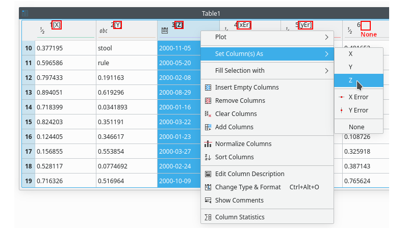
Columns can be assigned the following flags: X, Y, Z, X-error, Y-error or can be simple columns without any special flag(None). The X columns are abscissae columns while the Y columns are ordinate columns used when creating a 2D plot from data. The Z columns are used for 3D plots. The X-error and Y-error columns can be used in order to add error bars to 2D plots.
The line color in the column header also represents the flag X(green), Y(brown), Z(violet), X-error/y-error(red), none(grey).
Type/Format Lock
The assigned flag or type will be locked(depicted by the lock symbol along with the type icon) once you use the column for 2D or 3D plots. After locking, the user will not be allowed to change the type/format unless the plot associated with the column doesn't exist anymore.
Operations
You can select all the columns of the spreadsheet (Ctrl+A) or only some of them by clicking on the column label while keeping the Ctrl key pressed, or by moving the mouse over the column label. This also allows you to deselect columns.
On the selected columns you can perform various operations:
- Fill with data. You can insert the row numbers (Fill Selection With→Row Numbers command), random numbers (Fill Selection With→Random Values command), custom random numbers(Fill Selection With→Custom Random Values command and select Gaussian, Laplace, Exponential distributions etc), or the result of a function (Assign Formula command);
- normalize columns with the Normalize Columns command of the context menu;
- sort columns with the Sort Table command of the Table menu or with the sort column command of the context menu;
- compute statistical data on columns and rows with the Statistics on Columns command and Statistics on Rows command of the Analysis-tables menu;
- build a plot from selected columns with the plot command of the context menu or with the commands of the Plot menu
All these functions can be reached by right-clicking when a column is selected. Most of them can also be reached by using the Table menu.
You can cut, copy and paste data between spreadsheets or between a spreadsheet and another application (Excel, Gnumeric, OpenOffice Calc, etc).
You can import single or multiple ASCII files using the Import Ascii command from the File menu. This will create one or more new tables. You can also export the data from the spreadsheet to a text file using the Export Ascii command.
Import ASCII
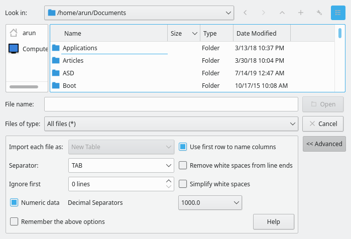
Imports one or more ASCII files (File -> Import Ascii) into the project by creating a new table storing the data from the file.
You can choose to put each data file in a separate table or join all the data files in one table. There is no automatic analysis of the data. Therefore, by default, the data will be read as text. If you want to obtain directly numeric values, you can specify it in the numeric data checkbox. You must then indicate the format of the numbers. The other possibility is to read data as text and then to specify the type and format of the different columns with the properties dialog of the tables.
If you check the Remember the above options, the selected parameters will be used as default values. They will be used if you read an ASCII file directly from the command line (see the Command line options section for more details).
- File: New document, New Table, New Matrix, New Graph, New 2D Plot, New 3D Plot, Open..., Open Recent, Close, Close All, Save, Save As..., Save a Copy..., Save All, Revert, Import..., Export..., Merge project..., Document information..., Print..., Print preview..., Export PDF...Exit
- Edit: Undo, Redo, Cut, Copy, Paste, Duplicate selection, Refresh, Select All, Delete, Preferences...
- View: Fullscreen, Workbench, Sync view, Record selection, Single document, Multi document, Collapse/Expand, Initiate dragging, Go to selection, Selection back, Selection forward, Status bar
- Tools: Edit parameters..., Export dependency graph..., Project utility..., Alphaplot, Line, Scatter, Scatter, Scatter With X Err, Scatter With Y Err, Scatter With XY Err, Line + Symbol, Special Line + Symbol, Vertical Drop Lines, Spline, Vertical Steps, Horizontal Steps, Vertical Bars, Vertical Stacked Bars, Vertical Grouped Bars ,Horizontal Bars, Horizontal Stacked Bars, Horizontal Grouped Bars, Area, Channel Fil, Pie, Half Pie, Vectors XYXY, Vectors XYAM, Statistical Graph, Box Plot, Histogram, Stacked Histogram, 3D Plot, Bar, Scatter, Layout Grids, Vertical 2 Layouts, Horizontal 2 Layouts, 4(2x2) Layouts, 3D Wire Frame, 3D Surface, 3D Wire Frame Surface, Bar, Scatter, Contour + Color Fill, Countour Lines, Gray Scale Map, 3D Wire Frame Polar, 3D Surface Polar, 3D Wire Frame Surface Polar, 3D Scatter Polar, Polar spectrogram, Graph, Add/Remove Plot xy/xy..., Add Function..., Add Error Bars..., Add/Remove Other Plots..., Add/Remove Plot y..., Add/Remove Vector Plot..., Add Axis..., Add Left Axis, Add Bottom Axis, Add Right Axis, Add Top Axis, Legend Reorder, Add Text, Add Time Stamp, Add Image, Draw Line, Draw Arrow, Draw Ellipse, Add Nested Layout, Add Layout, Add Up, Add Down, Add Left, Add Right, Remove Layout, Swap Layouts..., Graph Tolls, Disable Tools, Data Rearder, Screen Reader, Select Data Range, Move Data Points, Remove Bad Data Points..., Drag Range, Zoom Range, Rescale To Show All, Table, Set Column(s) As, X, Y, Z, X Error, Y Error, None, Fill Selection With, Row Numbers, , Random Values, Custom Random, Show Comments, Show Controls, Formula Edit Mode, Edit Column Description, Change Type & Format, Clear Table, Sort Table, Assign Formula, Recalculate, Add Column, Go To Cell, Export ASCII..., Convert To Matrix, Matrix, Hide Controls, Set Coordinates, Set Display Format, Assign Formula, Recalculate, Clear Matrix, Transpose, Mirror Horizontally, Mirror Vertically, Import Image, Go To Cell, Invert, Determinant, Convert To Table, Add text document, Group, Units Calculator,Customize..., RPS Features..., Addon manager
- Macro: Macro recording, Macros, Recent macros, Execute macro, Attach to remote debugger, Debug macro, Stop debugging, Step over, Step into, Toggle breakpoint
- Help: Help, LabRPS Website, Donate, Users documentation, Python scripting documentation, Automatic Python modules documentation, LabRPS Forum, LabRPS FAQ, Report a bug, About LabRPS, What's This
- Getting started
- Installation: Download, Windows, Linux, Mac, Additional components, AppImage
- Basics: About LabRPS, Interface, RPS Objects, Object name, Preferences, Workbenches, Document structure, Properties, Help LabRPS, Donate
- Help: Tutorials, Video tutorials
- Workbenches: Std Base, WindLab, SeismicLab, SeaLab, UserLab, Spreadsheet, Plot, Web
- Hubs: User hub, Power users hub, Developer hub


