Interpolation

Given a set of data points (x₁, y₁) ... (x_n, y_n) the routines described in this section compute a continuous interpolating function y(x) such that y(x_i) = y_i. The interpolation is piecewise smooth, and its behavior at the end-points is determined by the type of interpolation used.

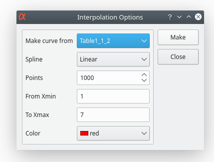
Interpolation will create a new data plot with a high number of points by interpolation of your data. The dialog box allows us to define this number of points (default value = 1000). Then the method used for interpolation, the interval of X-values, and the color of the interpolated curve can be chosen. In addition to the new curve in the active plot, a new table will be created.

Types

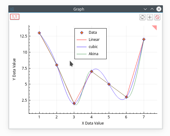
The simplest interpolation method is the linear method. In this case, a linear variation is used to compute the data points between two values. The cubic method will use the Cubic Splines method. Akima is a form of polynomial interpolation. You can refer to the corresponding section of the GNU Scientific Library for more details.

The interpolation method provides the following interpolation types:

Linear

If the two known points are given by the coordinates (x₀ , y₀) and (x₁ , y₁), the linear interpolant is the straight line between these points.

Polynomial

This method should only be used for interpolating small numbers of points because polynomial interpolation introduces large oscillations, even for well-behaved datasets. The number of terms in the interpolating polynomial is equal to the number of points.

Cubic

Cubic spline with natural boundary conditions. The resulting curve is piecewise cubic on each interval, with matching first and second derivatives at the supplied data-points. The second derivative is chosen to be zero at the first point and last point.

Cubic Periodic

Cubic spline with periodic boundary conditions. The resulting curve is piecewise cubic on each interval, with matching first and second derivatives at the supplied data-points. The derivatives at the first and last points are also matched. Note that the last point in the data must have the same y-value as the first point, otherwise the resulting periodic interpolation will have a discontinuity at the boundary.

Akima

Non-rounded Akima spline with natural boundary conditions. This method uses the non-rounded corner algorithm of Wodicka.

Akima Periodic

Non-rounded Akima spline with periodic boundary conditions. This method uses the non-rounded corner algorithm of Wodicka.

Steffen

Steffen’s method guarantees the monotonicity of the interpolating function between the given data points. Therefore, minima and maxima can only occur exactly at the data points, and there can never be spurious oscillations between data points. The interpolated function is piecewise cubic in each interval. The resulting curve and its first derivative are guaranteed to be continuous, but the second derivative may be discontinuous.