WindLab Tutorial GeorgeDeodatis 1996 Example SimulationPoints

Tutorial
Topic
Wind Simulation Points (George Deodatis, 1996)
Level
Beginner
Time to complete
10 minutes
Authors
Koffi Daniel
LabRPS version
0.1.0 or above
Example files
None
See also
None

Introduction

Deodatis (1996) provides a comprehensive method for simulating ergodic wind velocity time histories by modeling the wind as a stationary random process with well-defined statistical properties. His approach is particularly focused on multivariate wind simulations (i.e., for multiple correlated wind components at different locations in space. These locations where the wind velocity components are considered in space are called Simulation Point in WindLab. This example is meant to show how a wind simulation points in LabRPS's WindLab Workbench looks like in the LabRPS interface and how their coordinates can be visualized. Every computation in LabRPS needs a RPS Feature. Here we rather need a WindLab Feature (RPS Feature) which is should be provided by a plugin.

Requirements

• A compatible version of LabRPS designated in the tutorial overview.

  Use the Help → About LabRPS to see the version of LabRPS installed.

• No external software is needed for the computation of the locations coordinates as well as for visualizing the results.
• Install the plugin that will provide the feature for the computation of the locations coordinates.

Plugin Installation

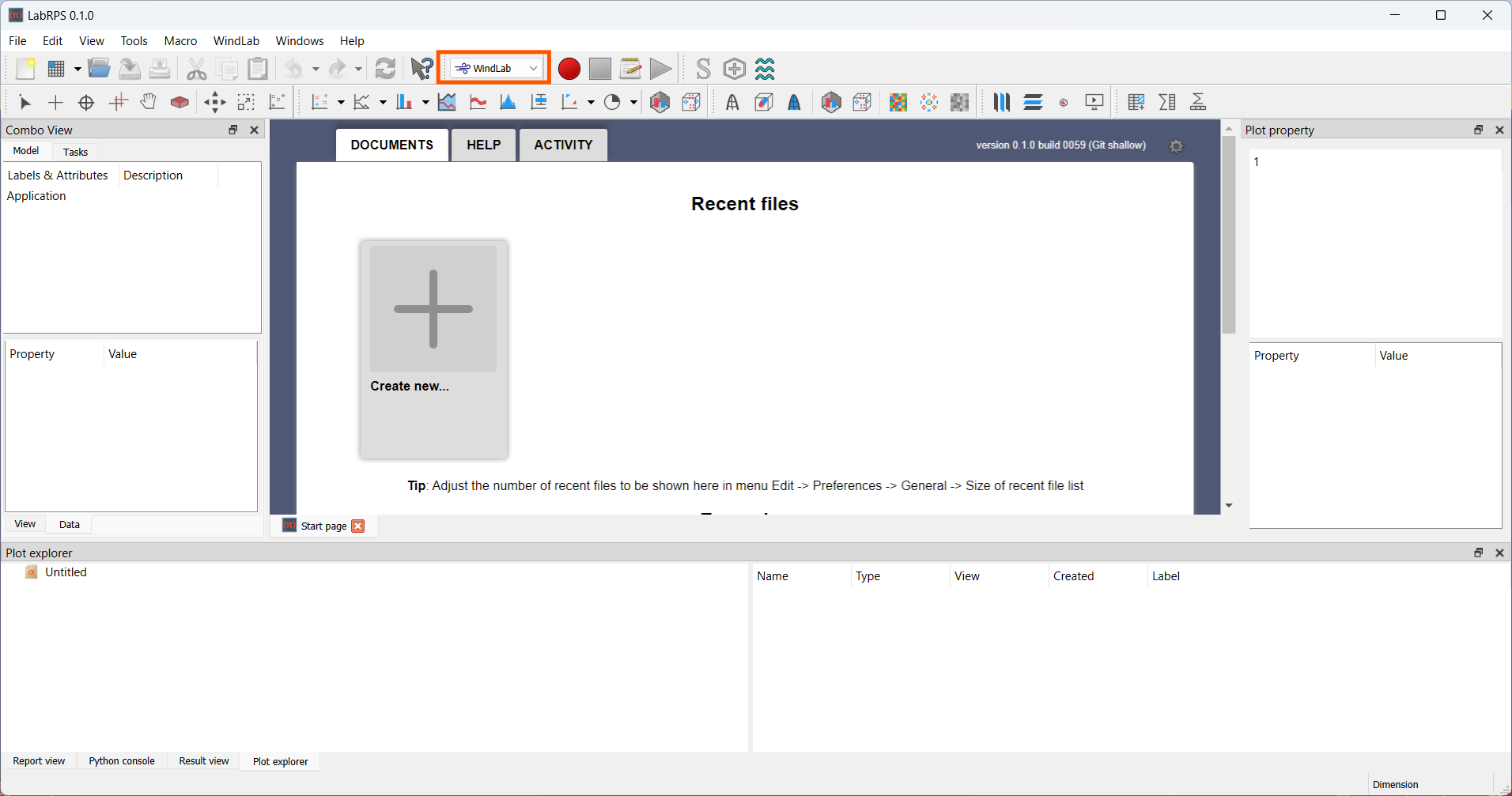
The first step is to start LabRPS by double-cliking its icon. Then active the WindLab workbench as shown in the following picture. Note that plugins are loaded according to the active workbench. If you do not activate the WindLab workbench, no wind velocity related plugin will be loaded.

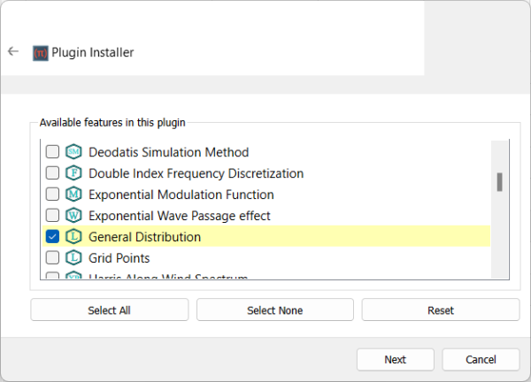
According to Deodatis (1996), the simulation points are three in total and their distribution in space does not follow any particular distribution in space. To compute such simulation distribution, the feature General Distribution from the WindLab Plugin. Let's install the feature first. Go to Tools → Feature Manager..., select the WindLabPlugin in the list and click Install as shown in the following picture.

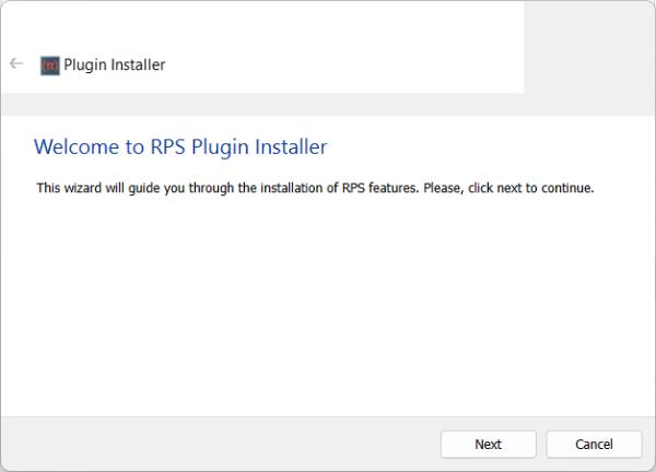
The Feature installation wizard will be launched. Please install the feautre by following the steps as shown in the following pictures:

Load the example file

• Start LabRPS.
• If the Start Workbench is not activated, load it and open the start page.
• Open the example "FemCalculixCantilever3D.FcStd".

Activate the analysis container

• To work with an analysis the analysis has to be activated.
• In the tree view, double click on the File:WindLab Analysis.svg Analysis,
• or right click on the File:WindLab Analysis.svg Analysis and choose Activate analysis.

Analysis container and its objects

• If the analysis is activated, LabRPS itself will change the current workbench to WindLab.
• There are at least 5 objects needed to make a static mechanical analysis.
• File:WindLab Analysis.svg analysis container

1. File:WindLab SolverCalculixCxxtools.svg a solver
2. File:WindLab MaterialSolid.svg a material
3. File:WindLab ConstraintFixed.svg a fixed boundary condition
4. File:WindLab ConstraintForce.svg a force load
5. File:WindLab WindLabMesh.svg a WindLab mesh

• In this example, results File:WindLab ResultShow.svg are already included as well.

Visualizing Results

1. Be sure the analysis is activated.
2. Be sure the analysis still contains the result object, if not just reload the example file.
3. Double click the result object File:WindLab ResultShow.svg, or select it and click the File:WindLab ResultShow.svg Show result button in the WindLab toolbar.
4. In the task window, choose z-Displacement. It shows -86.93 mm in negative z-direction. This makes sense since the force is in negative z-direction as well.
5. Activate the check box besides the bottom slider of displacement show.
6. The slider can be used to alter the mesh to view the deformation in a simplified manner.
7. Choose among the different Result types to view all in the GUI available result types.

Purging Results

1. Be sure the analysis is activated.
2. To remove the results: select in the icon toolbar the File:WindLab ResultsPurge.svg Purge results button.

Running the FEA

• In the tree view double click on the solver object File:WindLab SolverCalculixCxxtools.svg.
• In the task panel of the solver object make sure static analysis is selected.
• Click on Write .inp file in the same task window. Watch the log window until it prints "write completed."
• Click on Run CalculiX. Since this is a very small analysis it should take less than a second to run.
• In the text window it should print in green letters "CalculiX done without error!" and in the next line "loading result sets ..."
• You just have finished your first FEA in LabRPS if there has not been any error message.
• Click on Close in the task window.
• A new result object should be created. You know how to visualize the results already.
• If you get an error message no solver binary or similar when triggering the analysis check WindLab Install.

Running the FEA the fast Way

• In tree view select the solver object File:WindLab SolverCalculixCxxtools.svg of the analysis File:WindLab Analysis.svg.
• In the icon toolbar click on File:WindLab SolverRun.svg Run solver calculations.
• The Calculix input file will be written, CalculiX will be triggered and the result object should be created.

Changing Load Direction and Load Value

• In the tree view expand File:WindLab ResultShow.svg CCX_Results and select the File:WindLab MeshResult.svg ResultMesh object and press the Space key.
  • Result: The visibility of the WindLab mesh will be turned off. The geometrical model is still visible.
• In the tree view double click on the File:WindLab ConstraintForce.svg WindLabConstraintForce object to open its task panel
• In the task window change the load value to 500000000 N = 500 MN (Note: force unit in task window has to be in N)
• On the geometrical model click on one of the long edges in x-direction.
• Click on the Direction button.
  • Result: The red arrows that illustrate force will change their direction in x-direction. They indicate the force direction.
• Since tension should be applied to the box the Reverse Direction needs to be triggered by clicking on it.
• The red arrows of the force will change their direction.
• Click on OK in task window.

• You know how to trigger an analysis and how to visualize results already.
• The deformation in x-direction should be 18.95 mm.

What next?

• We are now finished with the basic workflow for the WindLab Workbench.
• You are now prepared to do the second WindLab tutorial.
• We will create the CalculiX cantilever by ourselves and compare the results with the beam theory.

WindLab

• WindLab: New Simulation, WindLab Features

User documentation

• Getting started
• Installation: Download, Windows, Linux, Mac, Additional components, AppImage
• Basics: About LabRPS, Interface, RPS Objects, Object name, Preferences, Workbenches, Document structure, Properties, Help LabRPS, Donate

---

• Help: Tutorials, Video tutorials
• Workbenches: Std Base, WindLab, SeismicLab, SeaLab, UserLab, Spreadsheet, Plot, Web

---

• Addons: Addon Manager, Plugins, Scripting and macros

---

• Hubs: User hub, Power users hub, Developer hub