WindLab Tutorial GeorgeDeodatis 1996 Example SimulationPoints: Difference between revisions
(Created page with "{{TutorialInfo |Topic=Wind Simulation Points (George Deodatis, 1996) |Level=Beginner |Time=10 minutes |Author=[https://wiki.labrps.com/User:LabRPS Koffi Daniel] |RPSVersion=0.1.0 or above }} == Introduction == Deodatis (1996) provides a comprehensive method for simulating ergodic wind velocity time histories by modeling the wind as a stationary random process with well-defined statistical properties. His approach is particularly focused on multivariate wind simulation...") |
No edit summary |
||
| Line 35: | Line 35: | ||
[[Image:WindLab_Tutorial001_Pic003_WindLab_Wizard_3.png|600px]] [[Image:WindLab_Tutorial001_Pic003_WindLab_Wizard_4.png|600px]] | [[Image:WindLab_Tutorial001_Pic003_WindLab_Wizard_3.png|600px]] [[Image:WindLab_Tutorial001_Pic003_WindLab_Wizard_4.png|600px]] | ||
== | == Create New Feature == | ||
Please follow the following steps to create new WindLab simulation and add new Location distribution feature to it. | |||
[[Image: | # Press the {{Button|[[Image:Std_New.svg|16px]] [[Std_New|New]]}} button to create new document or | ||
#* Select the {{MenuCommand|File → [[Image:Std_New.svg|16px]] New}} option from the menu or | |||
#* Use the keyboard shortcut: {{KEY|Ctrl}}+{{KEY|N}}. | |||
# Press the {{Button|[[Image:WindLab_CreateSimulation.svg|16px]] [[WindLab_CreateSimulation|New Simulation]]}} button to create new WindLab simulation or | |||
#* Select the {{MenuCommand|WindLab → [[Image:WindLab_CreateSimulation.svg|16px]] New Simulation}} option from the menu. | |||
#* This will display the WindLab simulation creation task dialog as follows: | |||
[[Image:WindLab_Tutorial001_Pic004_WindLab_Sim_Creation_1.png|400px]] [[Image:WindLab_Tutorial001_Pic004_WindLab_Sim_Creation_2.png|400px]] [[Image:WindLab_Tutorial001_Pic004_WindLab_Sim_Creation_3.png|400px]] | |||
# Press the {{Button|[[Image:WindLab_CreateFeature.svg|16px]] [[WindLab_CreateFeature|Create Feature]]}} button to create new Location Distribution feature or | |||
#* Select the {{MenuCommand|WindLab → [[Image:WindLab_CreateFeature.svg|16px]] Create Feature}} option from the menu. | |||
* | |||
[[Image: | [[Image:WindLab_Tutorial001_Pic004_WindLab_Sim_Creation_3.png|400px]] [[Image:WindLab_Tutorial001_Pic004_WindLab_Feat_Creation_1.png|400px]] [[Image:WindLab_Tutorial001_Pic004_WindLab_Feat_Creation_2.png|400px]] | ||
== | == Input Points Coordinates == | ||
== Showing Results == | |||
= | |||
== What next? == | == What next? == | ||
* We are now finished with the basic workflow for the [[WindLab_Workbench|WindLab Workbench]]. | * We are now finished with the basic workflow for the [[WindLab_Workbench|WindLab Workbench]] feature creation. | ||
* You are now prepared to do the second [[ | * You are now prepared to do the second [[WindLab_Tutorial_GeorgeDeodatis_1996_Example_MeanWindProfile|WWindLab tutorial]]. | ||
* We will create the | * We will create meand wind profile that will use the simulation points coordinates created in this tutorial. | ||
{{WindLab Tools navi}} | {{WindLab Tools navi}} | ||
{{Userdocnavi}} | {{Userdocnavi}} | ||
Revision as of 19:47, 14 November 2024
| Topic |
|---|
| Wind Simulation Points (George Deodatis, 1996) |
| Level |
| Beginner |
| Time to complete |
| 10 minutes |
| Authors |
| Koffi Daniel |
| LabRPS version |
| 0.1.0 or above |
| Example files |
| None |
| See also |
| None |
Introduction
Deodatis (1996) provides a comprehensive method for simulating ergodic wind velocity time histories by modeling the wind as a stationary random process with well-defined statistical properties. His approach is particularly focused on multivariate wind simulations (i.e., for multiple correlated wind components at different locations in space. These locations where the wind velocity components are considered in space are called Simulation Point in WindLab. This example is meant to show how a wind simulation points in LabRPS's WindLab Workbench looks like in the LabRPS interface and how their coordinates can be visualized. Every computation in LabRPS needs a RPS Feature. Here we rather need a WindLab Feature (RPS Feature) which is should be provided by a plugin.
Requirements
- A compatible version of LabRPS designated in the tutorial overview.
- Use the Help → About LabRPS to see the version of LabRPS installed.
- No external software is needed for the computation of the locations coordinates as well as for visualizing the results.
- Install the plugin that will provide the feature for the computation of the locations coordinates.
Plugin Installation
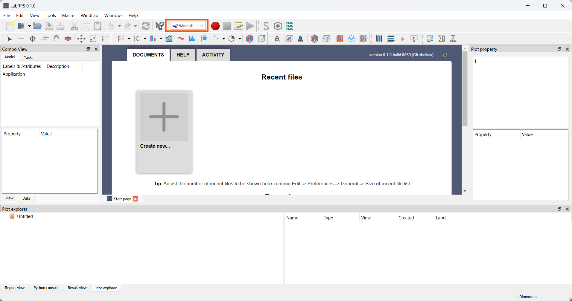
The first step is to start LabRPS by double-cliking its icon. Then active the WindLab workbench as shown in the following picture. Note that plugins are loaded according to the active workbench. If you do not activate the WindLab workbench, no wind velocity related plugin will be loaded.
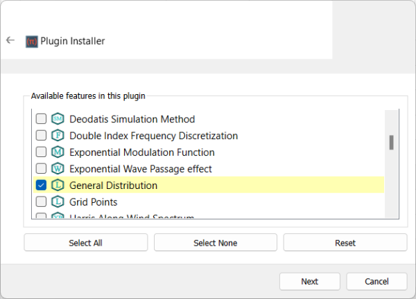
According to Deodatis (1996), the simulation points are three in total and their distribution in space does not follow any particular distribution in space. To compute such simulation distribution, the feature General Distribution from the WindLab Plugin. Let's install the feature first.
Go to Tools → Feature Manager..., select the WindLabPlugin in the list and click Install as shown in the following picture.
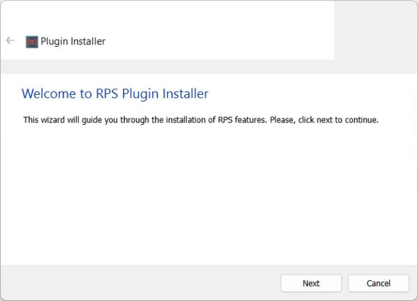
The Feature installation wizard will be launched. Please install the feautre by following the steps as shown in the following pictures:
Create New Feature
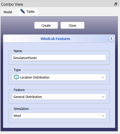
Please follow the following steps to create new WindLab simulation and add new Location distribution feature to it.
- Press the
New button to create new document or
- Press the
New Simulation button to create new WindLab simulation or
- Press the
Create Feature button to create new Location Distribution feature or
Input Points Coordinates
Showing Results
What next?
- We are now finished with the basic workflow for the WindLab Workbench feature creation.
- You are now prepared to do the second WWindLab tutorial.
- We will create meand wind profile that will use the simulation points coordinates created in this tutorial.
- Getting started
- Installation: Download, Windows, Linux, Mac, Additional components, AppImage
- Basics: About LabRPS, Interface, RPS Objects, Object name, Preferences, Workbenches, Document structure, Properties, Help LabRPS, Donate
- Help: Tutorials, Video tutorials
- Workbenches: Std Base, WindLab, SeismicLab, SeaLab, UserLab, Spreadsheet, Plot, Web
- Hubs: User hub, Power users hub, Developer hub


