Plugin WindLab SimulatedSpectrumTool

Simulated Spectrum Tool Plugin
Description
This plugin computes the power spectral density function the simulated wind velocities. Plugin version: 1.0 Last modified: 15/01/2025 LabRPS version: All Author: Koffi Daniel
Author
Koffi Daniel
Download
None
Features
Simulated Spectrum Tool
Plugin Version
1.0
Date last modified
15/01/2025
LabRPS Version(s)
All
Default shortcut
None
See also
None

Introduction

This plugin computes the power spectral density function the simulated wind velocities.

Simulated Spectrum Tool

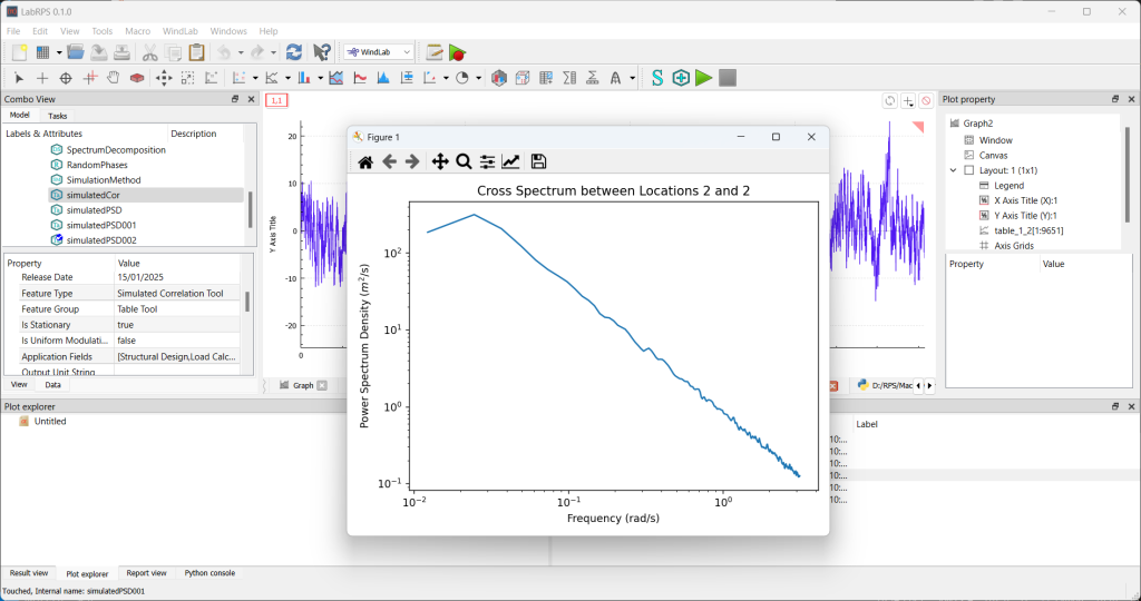
This is the only RPS feature that the plugin implements. It belongs to the table tool group. This feature uses the simulated wind velocity to compute the power spectral density function. Therefore, you need to make sure you simulate random wind velocity first. You can also import the wind velocity from file. Note that if you use the mouse (GUI mode) to run this feature, you have to make sure the active window is the window containing the wind velocity data for which you want to compute the temporal correlation.

Properties

• DatafftPointsNumber: This number of DFT points used during the computation.
• DataWindowLength: The length of the window used to divide the two wind processes into segments and perform windowing.
• DataOverLap: The number of overlapped samples, specified as a positive integer.
• DataWindowType: This is the type of windowing.

Scripting

import LabRPS
import WindLabObjects
import WindLabGui
import WindLab
import GeneralToolsGui

# Before you run this macro, simulation must be run and there  must be a table containing the simulated wind velocities.
def checkResult():
    # Install the ergodicity checking tool
    installResuslt = WindLab.installPlugin("SimulatedSpectrumToolPlugin")
    if not installResuslt:
        LabRPS.Console.PrintError("The installation of the SimulatedSpectrumToolPlugin has failed.\n")
        return None

    # Get the active simulation which as this time has been run already.   
    sim = WindLabGui.getActiveSimulation()

    # get the simulation data as list assuming that a wind simulation is run and 
    # the result is shown in an AlphaPlot table called "table". Please, edit this table name
    # according to the name of the table where your simulated data are stored.
    velocities = GeneralToolsGui.GeneralToolsPyTool.getTableByName("table")

    # create new table tool
    simulatedPSD = WindLabObjects.makeFeature("simulatedPSD", sim.Name, "Simulated Spectrum Tool", "Table Tool")
    
    # check if the created randomness provider feature
    if not simulatedPSD:
        LabRPS.Console.PrintError("The creation of the table tool was not successuful.\n")
        return None
    simulatedPSD.WindowType = "Hamming window"
    sim.setActiveFeature(simulatedPSD)        
    simulatedPSDRest = sim.tableToolCompute(velocities)

    # if we are in Gui mode, show the plot
    if LabRPS.GuiUp:
        fftl = simulatedPSD.fftPointsNumber//2
        # GeneralToolsGui.GeneralToolsPyTool.tablePlotCurve(len(simulatedPSDRest), fftl+1, simulatedPSDRest, 0, 1)    

        import numpy
        import matplotlib.pyplot as plt

        # convert the list to numpy array
        array = numpy.asarray(simulatedPSDRest)
        locationJ = sim.LocationIndexJ + 1
        locationK = sim.LocationIndexK + 1
        str1 = "{:d}".format(locationJ)
        str2 = " and {:d}".format(locationK)
        str = "Cross Spectrum between Locations " + str1 + str2
        fig, ax = plt.subplots()
        ax.set_title(str)
        f = sim.getSimulationData().numberOfFrequency - 1 
        ax.plot(array[0:fftl,0], array[0:fftl,1])
        ax.set_xlabel('Frequency (rad/s)')
        ax.set_ylabel('Power Spectrum Density ($m^2$/s)')
        # ax.grid(True)
        ax.set_xscale("log")
        ax.set_yscale("log")
        fig.tight_layout()
        plt.show()

checkResult()