Fast Fourier Transform(FFT)
A fast Fourier transform (FFT) is an algorithm that computes the discrete Fourier transform (DFT) of a sequence. Fourier analysis converts a signal from its original domain (often time or space) to a representation in the frequency domain.
This function can be accessed by the FFT command of the Analysis-tables menu when a table is selected, or Analysis-plots menu when a plot is selected. The Fourier transform decomposes a signal in its elementary components by assuming that the signal x(t) can be described as a sum:
in which ωn are the frequencies, an are the amplitudes of each frequency and ψn are the phase corresponding frequency. LabRPS will compute these parameters and build a new plot of the amplitude as a function of the frequency. FFT can be performed on a curve to extract the characteristic frequencies.
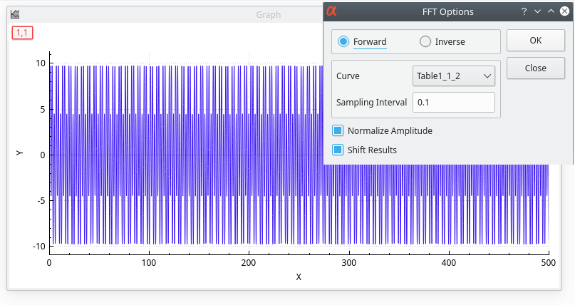
Let's assume you have the signal presented in the next figure. You can select the FFT command of the Analysis-plots menu to open the FFT dialog box.
If the Normalize Amplitude checkbox is on, the amplitude curve is normalized to 1. If the Shift Results checkbox is on, the frequencies are shifted in order to obtain a centered x-scale. By default, the Sampling Interval corresponds to the interval between X-values. Giving a smaller value makes no sense, but you can increase this value in order to sample fewer values.
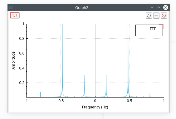
LabRPS will create a new plot window with the FFT amplitude curve, and a new table which contains the real part, the imaginary part, the amplitude, and the angle of the FFT. In this example, the amplitude curve has been normalized, and the frequencies have been shifted to obtain a centered x-scale.
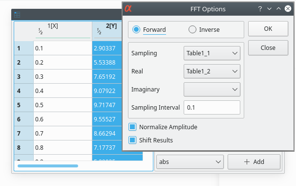
In the case of a table, you must select the sampling column (X-values) and one column (for real numbers) or two columns (for complex numbers) for Y-values.
Filtering of Signals
In this section, it will be assumed that you have the signal presented in the previous section (see figure Figure 3.1, “A signal and the FFT dialog box for a plot.”). We can analyze this signal by doing an FFT on the data curve and it will show that this signal has a power spectrum with high and low frequencies (see figure Figure 3.2, “The resulting FFT with the characteristic frequencies.”). The next sections will show the influence of the different filters on this signal.
Low pass filter
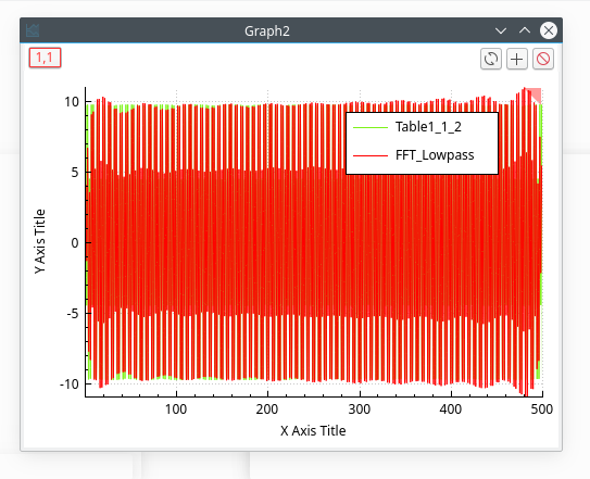
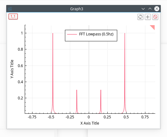
This filter allows us to cut the high frequencies of a signal. You just have to select the cut-off frequency of the filter. Let us assume that we want to keep the frequencies below 0.5 Hz, we will obtain:
The power spectrum of this new signal shows that the frequencies below 0.5 Hz have been kept.
High pass filter
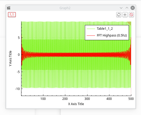
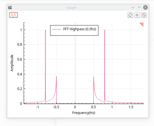
This filter allows us to cut the low frequencies of a signal. You just have to select the cut-off frequency of the filter. Let us assume that we want to keep the frequencies above 0.5 Hz, we will obtain:
The power spectrum of this new signal shows that the frequencies above 0.5 Hz have been kept.
Band pass filter
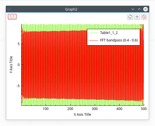
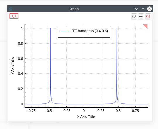
This filter allows us to cut the low and high frequencies of a signal. You just have to select the high and low cut-off frequencies of the filter. Let us assume that we want to keep the frequencies between 0.4 and 0.6 Hz, we will obtain:
The power spectrum of this new signal shows that only the frequencies at 0.4 and 0.6 Hz have been kept.
Block band filter
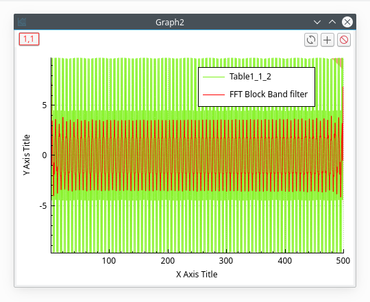
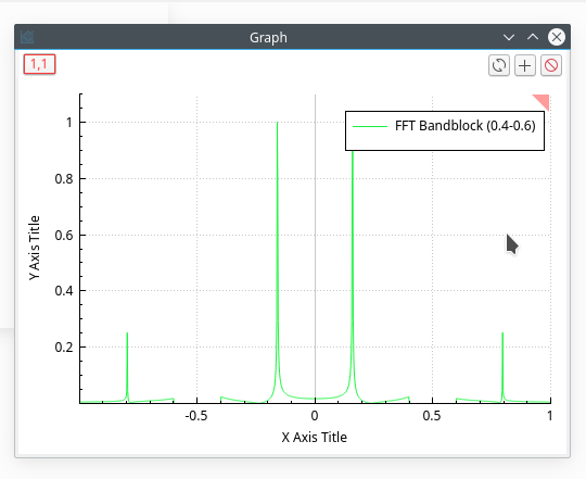
This filter allows us to keep the low and high frequencies of a signal. You just have to select the high and low cut-off frequencies of the filter. Let us assume that we want to remove the frequencies between 0.4 and 0.6 Hz, we will obtain:
The power spectrum of this new signal shows that only the frequencies below 0.4 Hz and above 0.6 Hz have been kept.

